The NVIDIA NGC team is hosting a webinar with live Q&A to dive into this Jupyter notebook available from the NGC catalog. Learn how to use these resources to kickstart your AI journey. Register now: NVIDIA NGC Jupyter Notebook Day: Image Segmentation.
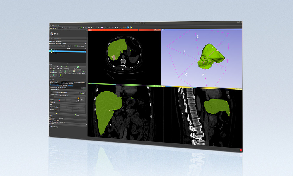
Image segmentation is the process of partitioning a digital image into multiple segments by changing the representation of an image into something that is more meaningful and easier to analyze. Image segmentation can be used in a variety of domains such as manufacturing to identify defective parts, in medical imaging to detect early onset of diseases, in autonomous driving to detect pedestrians, and more.
However, building, training, and optimizing these models can be complex and quite time consuming. To achieve a state-of-the-art model, you need to set up the right environment, train with the correct hyperparameters, and optimize it to achieve the desired accuracy. Data scientists and developers usually end up spending a considerable amount of looking for the right tools and setting up the environments for their models, which is why we built the NGC Catalog.
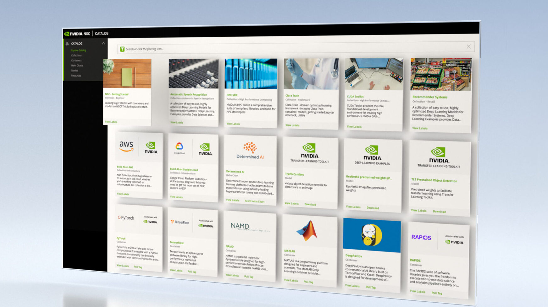
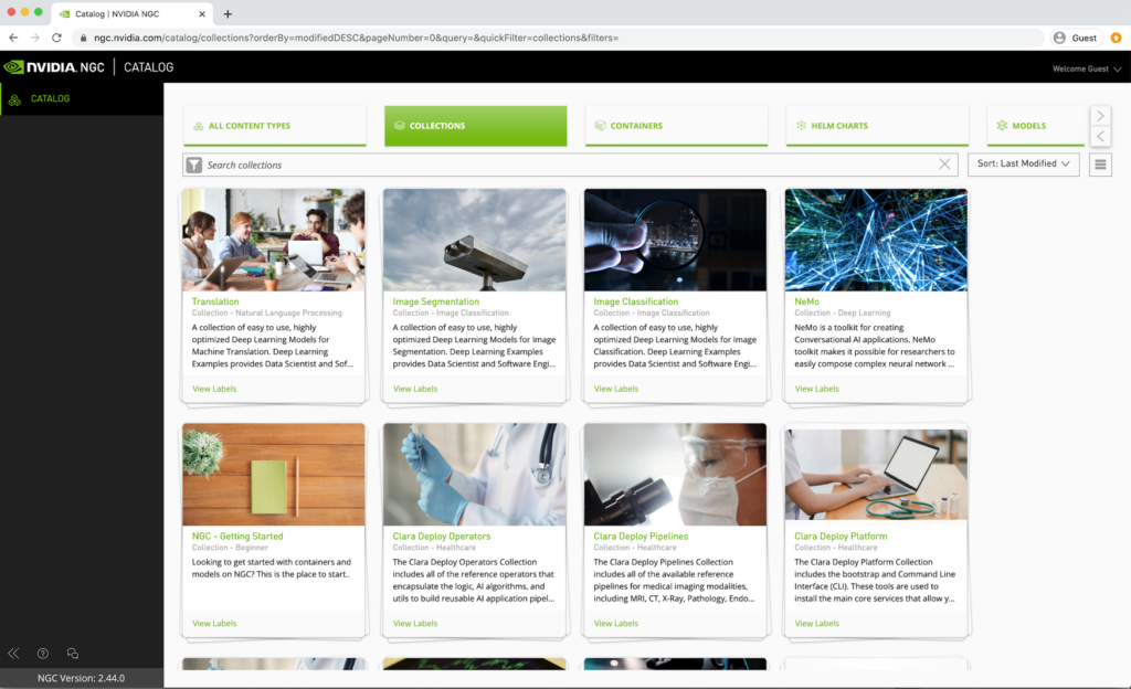
A hub for cloud-native, GPU-optimized AI and HPC applications and tools that provides faster access to performance-optimized containers, shortens time-to-solution with pretrained models and provides industry specific software development kits to build end-to-end AI solutions. The catalog hosts a diverse set of assets that can be used for a variety of applications and use cases ranging from computer vision and speech recognition to recommendation systems.
The AI containers and models on the NGC Catalog are tuned, tested, and optimized to extract maximum performance from your existing GPU infrastructure. The containers and models use automatic mixed precision (AMP), enabling you to use this feature with either no code changes or only minimal changes. AMP uses the Tensor Cores on NVIDIA GPUs and can speed up model training considerably. Multi-GPU training is a standard feature implemented on all NGC models that leverage Horovod and NCCL libraries for distributed training and efficient communication.
Aside from providing just the building blocks, NGC is now adding sample Jupyter notebooks complete with instructions on how to train and deploy a model using these artifacts from the NGC Catalog. In this post, I show you how to use a sample image segmentation notebook to identify defective parts in a manufacturing assembly line.
Image segmentation
This U-Net model is adapted from the original version of the U-Net model, which is a convolutional auto-encoder for 2D image segmentation. This work proposes a modified version of U-Net, called TinyUNet, which performs efficiently and with high accuracy on the industrial anomaly dataset DAGM2007. TinyUNet is composed of two parts, encoding and decoding subsystems. The encoder converts the input sequence into a single dimensional vector. The decoder uses the output of the encoder as input and converts this vector into the output sequence.
This model repeatedly applies three downsampling blocks composed of two 2D convolutions followed by a 2D max pooling layer in the encoding subnetwork. In the decoding subnetwork, three upsampling blocks are composed of a upsample2D layer followed by a 2D convolution, a concatenation operation with the residual connection, and two 2D convolutions.
This is the default configuration of the model:
- Epochs: 2500
- Global Batch Size: 16
- Optimizer RMSProp:
- decay: 0.9
- momentum: 0.8
- centered: True
- Learning Rate Schedule: Exponential Step Decay
- decay: 0.8
- steps: 500 initial
- learning rate: 1e-4
- Weight Initialization: He Uniform Distribution (introduced by Kaiming He et al. in 2015 to address issues related ReLU activations in deep neural networks)
- Loss Function:
- When DICE Loss < 0.3, Loss = Binary Cross Entropy
- Else, Loss = DICE Loss
- Data Augmentation:
- Random Horizontal Flip (50% chance)
- Random Rotation 90?°
- Activation Functions:
- ReLU is used for all layers Sigmoid is used at the output to ensure that the outputs are between [0, 1]
- Weight decay:
- 1e-5
This NGC resource contains a Dockerfile that extends the TensorFlow container in the NGC Catalog and encapsulates the necessary dependencies. Aside from these dependencies, you also need the following components:
- NVIDIA Docker
- TensorFlow 20.12-tf1-py3 NGC container
- Access to an NVIDIA GPU-based system
To train your model using mixed precision with Tensor Cores or using FP32, perform the following steps using the default parameters of the U-Net model on the EM segmentation challenge dataset. This enables you to build the U-Net TensorFlow NGC container, train and evaluate your model, and generate predictions on the test data.
Build the container
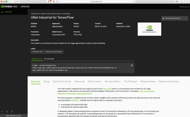
Find the U-Net model under the resources section in the NGC Catalog. You can download the resource manually from the top right menu or by using the wget resource command.
To build the container, follow these steps:
- Make a folder using
mkdir. - Go to that folder using
cd. - Use
wgetto download resources as a zip file inside the folder. - Unzip the zip file.
- Build the container using the Dockerfile inside this directory.
mkdir unet

cd unet

wget --content-disposition https://api.ngc.nvidia.com/v2/resources/nvidia/unet_industrial_for_tensorflow/versions/20.06.3/zip -O unet_industrial_for_tensorflow_20.06.3.zip
unzip unet_industrial_for_tensorflow_20.06.3.zip

docker build . --rm -t unet_industrial:latest
When you have built your container, follow the steps listed below to start an interactive session inside the NGC container:
- Make a directory for the dataset, for example ./dataset.
- Make a directory for results, for example ./results.
- Start the container with
nvidia-docker.
mkdir ./dataset

mkdir ./results

docker run -it --rm \
??? --shm-size=2g --ulimit memlock=-1 --ulimit stack=67108864 \
??? -v <absolute path to dataset directory that we made>:/data/ \
??? -v <absolute path to results directory that we made>:/results \
??? -p 8888:8888 unet_industrial:latest
Download and preprocess the data set
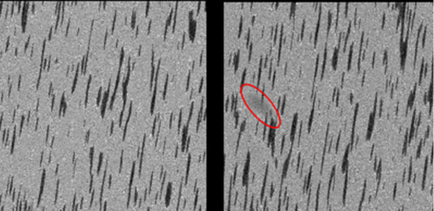
You use DAGM2007 dataset for training this model. This data set is artificially generated but is similar to real-world problems. It consists of multiple data sets, each consisting of 1000 images showing the background texture without defects and 150 images with one labeled defect each on the background texture. The images in a single data set are similar, but each data set is generated by a different texture model and defect model.
Figure 3 shows a sample image from this data set. The left image is without defect and the right image contains a scratch-shaped defect that appears as a thin dark line, and a diffuse darker area. The defects are labeled by a surrounding ellipse, shown in red.
To download the dataset, execute the following command. Some files in the dataset require an account. If you face a permissions problem while running any of these scripts, use chmod to add the scripts and rebuild the container.
chmod +x scriptname
For example:
chmod +x download_and_preprocess_dagm2007.sh
To download the dataset, run the following command:
./download_and_preprocess_dagm2007.sh /data
Download the rest of the data set
To download the complete dataset required for this tutorial, you can request access to the private data. The provided link allows you to download a group of 10 datasets to your local machine. For training and testing purposes, you must choose the class of data to use so you can download some of these datasets instead of all 10 classes.
When you have downloaded the dataset, open another terminal in your local machine. To copy downloaded files to your running container, run the following command in the terminal:
docker cp /home/<your file path> :/data/raw_images/private
An example command to copy class1 folder:
docker cp /home/skouchak/Class1.zip 1877b7cc7625:/data/raw_images/private
Unzip the folder using the following command:
unzip /folder/path/.zip
Start training
To train using the default configuration (for example 1/4/8 GPUs, FP32/TF-AMP), launch one of the scripts in the ./scripts directory:./scripts/UNet{AMP}{1, 4, 8}GPU.sh.
Each of the scripts requires several parameters:
- Path to the results directory of the model as the first argument
- Path to the dataset as a second argument
- Class ID from DAGM used (between 1-10)
For example, for class 1:
cd scripts/
./UNet_1GPU.sh /results /data 1
Run the evaluation
Launch model evaluation on a checkpoint by running one of the scripts in the ./scripts directory: ./scripts/UNet{_AMP}_EVAL.sh.
Each of the scripts requires three parameters:
- Path to the results directory of the model as the first argument
- Path to the dataset as a second argument
- Class ID from DAGM used (between 1-10)
cd scripts/
./UNet_EVAL.sh /results /data 1
Performance
In this section, you see how to benchmark the training and inference performance of the model using the related scripts.
Training performance benchmark
To benchmark the training performance, run one of the scripts in the ./scripts/benchmarking/ directory: ./scripts/benchmarking/UNet_trainbench{AMP}{1, 4, 8}GPU.sh. Each of the scripts requires two parameters:
- Path to the dataset as the first argument
- Class ID from DAGM used (between 1-10)
cd scripts/benchmarking/
./UNet_trainbench_1GPU.sh /data 1
Inference performance benchmark
To benchmark the inference performance, run one of the scripts in the ./scripts/benchmarking/ directory:./scripts/benchmarking/UNet_evalbench{_AMP}.sh.
Each of the scripts requires the following parameters:
- Path to the dataset as the first argument
- Class ID from DAGM used (between 1-10)
cd scripts/benchmarking/
./UNet_evalbench_AMP.sh /data 1
You can access the Jupyterlab notebook in the container by using the following command inside the container bash shell:
jupyter notebook --ip 0.0.0.0 --port 8888 --allow-root
Running the command results in a link to the Jupyterlab workspace in the container. Go to the workspace and upload the unet-industrial-demo notebook. Download the Jupyter notebook.
By following the unet-industrial-demo notebook, you can download 10 pretrained and fine-tuned models like the model that you just trained. You can test these models using images available in the public folders. To use the model that you trained instead of pretrained models, change the checkpoints folder path to the checkpoint of the model that you just trained and test your trained model using images in the public folder.
Advanced steps
The following sections provide greater details on the dataset, running training and inference and the results. To see the full list of available options and their descriptions, use the -h or --help command line option. For example:
python main.py --help
| General arguments | Description |
| –exec_mode=train_and_evaluate | Shows the execution mode. |
| –iter_unit=batch | Shows the number of batches and epochs. |
| –num_iter=2500 | Shows the number of iterations. |
| –batch_size=16 | Shows the size of each minibatch per GPU. |
| –results_dir=/path/to/results | Shows the directory in which to write training logs, summaries, and checkpoints. |
| –data_dir=/path/to/dataset | Shows the directory that contains the DAGM2007 dataset. |
| –dataset_name=DAGM2007 | Shows the name of the dataset used in this run. Only DAGM2007 is currently supported. |
| –dataset_classID=1 | Shows the ClassID to train or evaluate the network. This is used for DAGM. |
unet-industrial-demo notebook
After you have successfully trained the model, the next logical step is to deploy the model in production for inference. The UNet_Industrial TensorFlow checkpoint is trained with AMP. This model can be used for many different applications:
- Running inference/predictions using the model directly
- Building more efficient inference engines
- Resuming training from the downloaded checkpoint
- Transfer learning
- Training a student network
Download resources
Check your current path using the pwd command and adjust the path in the following command, including the path to the notebook folder of the resource that you just downloaded.
import os

WORKSPACE_DIR='/workspace/unet_industrial'
os.chdir(WORKSPACE_DIR)
print (os.getcwd())
Download some data for testing the Weekly Supervised Learning for Industrial Optical Inspection (DAGM 2007) competition dataset. To download the 10 public datasets for preprocessing, run the following command:
! ./download_and_preprocess_dagm2007_public.sh ./data
The next command downloads the model checkpoints as a zip file and unzips it:
wget --content-disposition https://api.ngc.nvidia.com/v2/models/nvidia/unet_industrial_tf_ckpt_amp/versions/19.08.0/zip -O unet_industrial_tf_ckpt_amp_19.08.0.zip
unzip unet_industrial_tf_ckpt_amp_19.08.0.zip
Upon completion of the download, the following model directories contain the pretrained models corresponding to the 10 classes of the DAGM 2007 competition data set:
!ls nvidia_unetindtf_fp16_20190522

Inference with native TensorFlow
In this section, you launch an interactive session to verify the correctness of the pretrained models, where you can load new test images.
Import some necessary libraries:
try:
    __import__("horovod")
except ImportError:
    os.system("pip install horovod")

import horovod.tensorflow
import sys

sys.path.insert(0,'/workspace/unet_industrial')
from model.unet import UNet_v1
import numpy as np
%matplotlib inline
import matplotlib.pyplot as plt
import matplotlib.image as mpimg
Select any image from the public image folders downloaded previously to test the model. You can choose any other image from these folders by changing the last two parts of the image address:
img = mpimg.imread('./data/raw_images/public/Class1_def/1.png')

plt.figure(figsize = (10,10));
plt.imshow(img, cmap='gray');
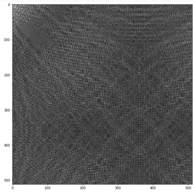
As you can see in Figure 5, there is a defective area in the top left corner. In the next step, you normalize the image:
# Image preprocessing
img.shape
img =  np.expand_dims(img, axis=2)
img =  np.expand_dims(img, axis=0)
img = (img-0.5)/0.5
img.shape
Testing the model
Restore the model using one of the checkpoints available in the /nvidia_unetindtf_fp16_20190522 folder (downloaded earlier). You can change the last three parts of the address to have access to other checkpoints.
import tensorflow as tf
import horovod.tensorflow as hvd
hvd.init()
config = tf.ConfigProto()
config.gpu_options.allow_growth = True
config.allow_soft_placement = True

graph = tf.Graph()
with graph.as_default():
    with tf.Session(config=config) as sess:
        network = UNet_v1(
            model_name="UNet_v1",
            input_format='NHWC',
            compute_format='NHWC',
            n_output_channels=1,
            unet_variant='tinyUNet',
            weight_init_method='he_uniform',
            activation_fn='relu'
        )

        tf_input = tf.placeholder(tf.float32, [None, 512, 512, 1], name='input')

        outputs, logits = network.build_model(tf_input)
        saver = tf.train.Saver()

        # Restore variables from disk.
        saver.restore(sess, "nvidia_unetindtf_fp16_20190522/Class 1/checkpoints/model.ckpt-2500")


        output = sess.run([outputs, logits], feed_dict={tf_input: img})
In the final step, plot the output of the model:
# Print out model predicted mask
plt.figure(figsize = (10,10))
plt.imshow(np.squeeze(output[0]), cmap='gray')
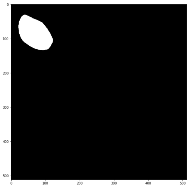
As expected, the model has captured the defective area in the image. Feel free to try out other defective images for Class 1 within ./data/raw_images/public/Class1_def/ or load the model and test data for other classes from 1 to 10.
Summary
In this post, I showed you how to use a sample image segmentation notebook to identify defective parts in a manufacturing assembly line using a Jupyter notebook from NGC.
Get started today by visiting the NGC Catalog, downloading the Jupyter notebooks for an image segmentation model and applying it to your own use cases.
NVIDIA GTC provides training, insights, and direct access to experts. Join us for breakthroughs in AI, data center, accelerated computing, healthcare, game development, networking, and more. Invent the future with us April 12-16, 2021.