Wireless networks are the essential infrastructure that enables seamless connectivity. To ensure the best performance, whether in a single building or a whole city, such networks are optimized using radio maps, which show the received signal strength across a large area, among other information.
Until now, the creation of radio maps was believed to be time-consuming, limiting the utility of sophisticated optimization methods. An NVIDIA research project has just established a new benchmark.
Differentiable radio maps in an instant
NVIDIA Instant Radio Maps (Instant RM) is a high-performance differentiable ray tracer that is capable of computing high-resolution radio maps at rates of about 100 maps per second. Built on rendering techniques from high-end computer graphics and adopting wireless propagation models, Instant RM uses NVIDIA hardware to its full potential to simulate radio wave propagation in large-scale and complex environments.
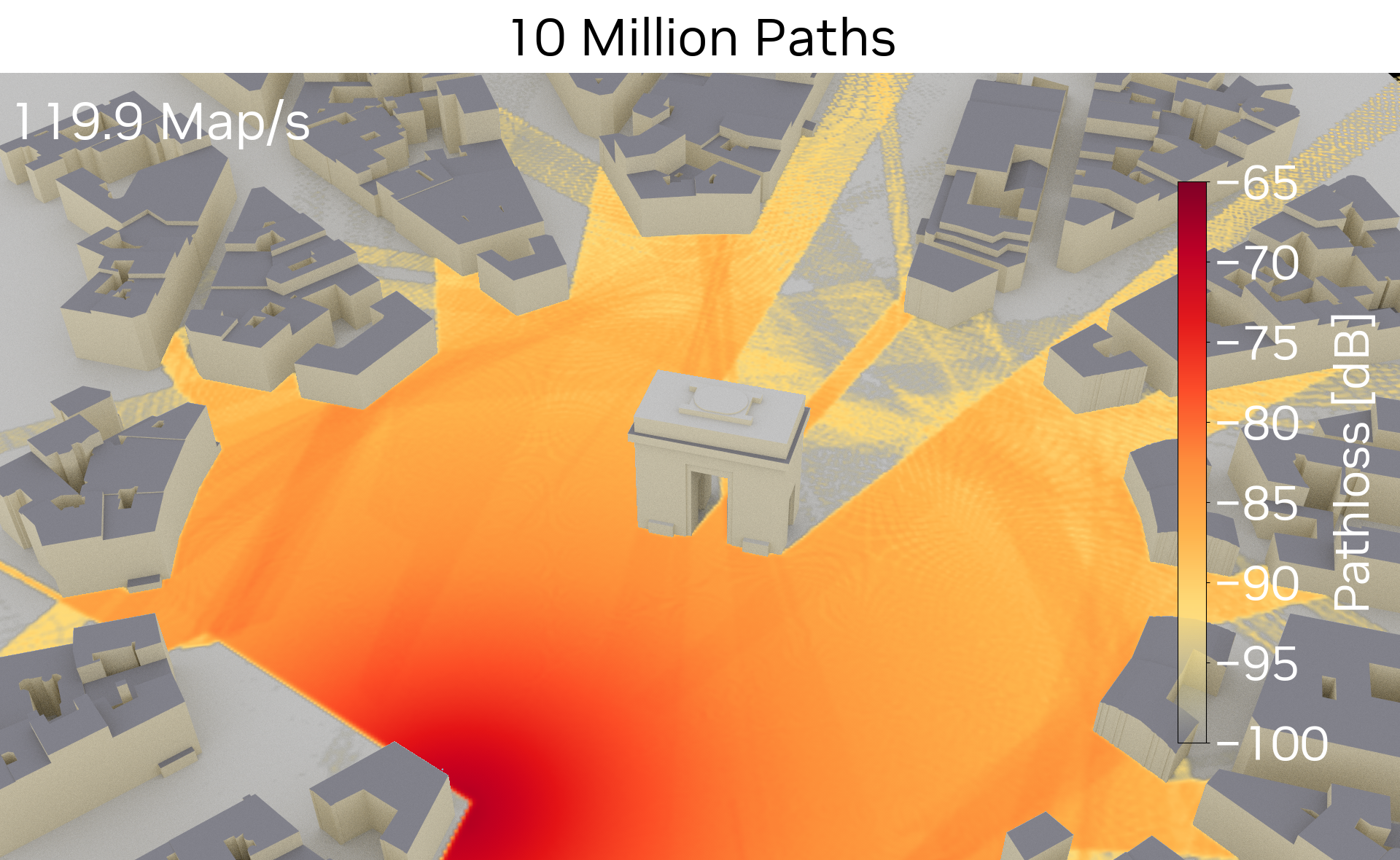
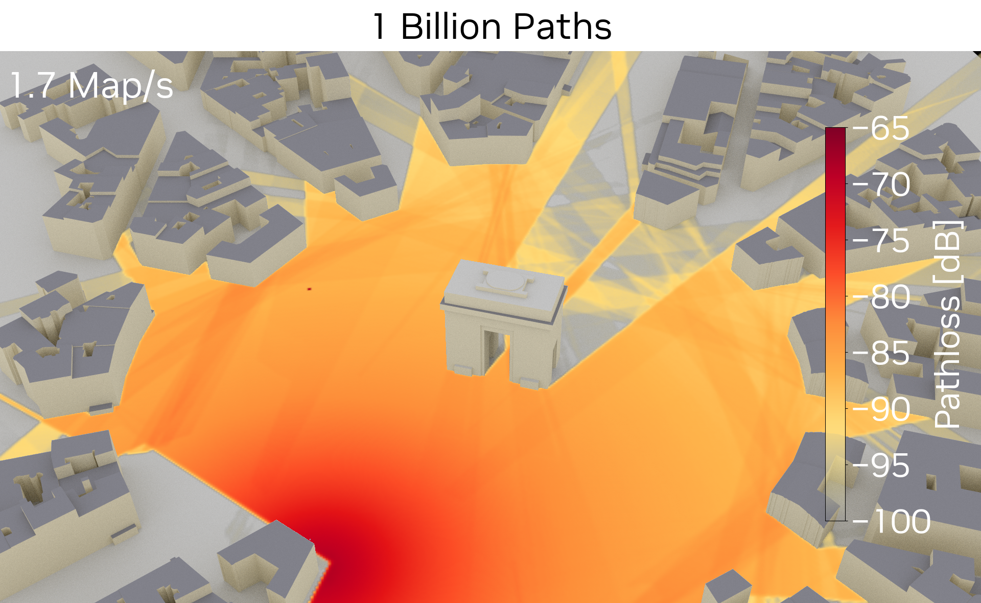
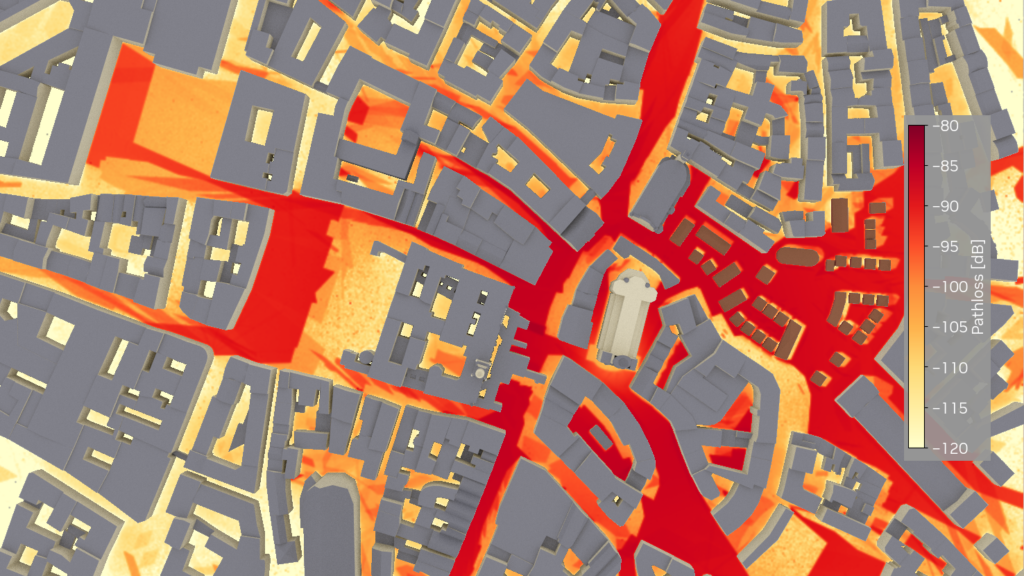
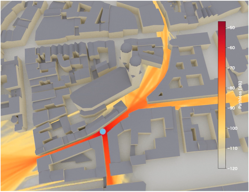
Figure 2 shows Paris near the Arc de Triomphe. The blue dot in each image indicates the location of a radio transmitter, and an overlaid radio map displays the path loss corresponding to this transmitter using a red-yellow color gradient. Some parts of the path loss map are noisy because of the relatively low number of samples used to compute it.
Instant RM reaches beyond path loss maps. It also supports the following:
- Computation of radio maps for the delay spread
- Direction spread of departure (DSD)
- Direction spread of arrival (DSA)
Such radio maps provide valuable information about the characteristics of the wireless channel.
The radio maps in Video 1 show path loss, delay spread, direction spread of arrival (DSA), and direction spread of departure (DSD) maps computed using Instant RM.
Instant RM only needs a few lines of code to load a scene, which defines the propagation environment, and to compute radio maps.
import mitsuba as miimport instant_rmimport numpy as np # Load the scenescene = mi.load_file("my_scene.xml") # Instantiate the map tracertracer = instant_rm.MapTracer(scene, # Carrier frequency [Hz] fc = 3.5e9, # Transmit antenna pattern tx_pattern = 'tr38901', # Slant angle [rad] tx_slant_angle = 0.0, # Radio map position, orientation, and size mp_center = np.array([0., 0., 1.5]), mp_orientation = np.array([0.,0.,0.]), mp_size = np.array([500.,500.]), # Size of a cell of the radio map mp_cell_size = np.array([1.,1.]), # Number of paths to compute the radio map num_samples = int(1e7), # Maximum number of interactions max_depth = 10) # Ray trace the radio maps# pm: Path loss map# rdsm: Root mean square delay spread map# mdam: Mean direction of arrival map# mddm: Mean direction of departure mappm, rdsm, mdam, mddm = tracer(# Transmitter position tx_position = np.array([0.,0.,20.]), # Transmitter orientation tx_orientation = np.array([np.pi, 0., 0.])) |
Let the gradients flow
Because Instant RM is a fully differentiable ray tracer, gradients of functions of the radio maps with respect to the material properties and the scene geometry can be readily computed.
An interesting application is the gradient-based calibration of a propagation environment from measurements, to ensure that simulation results match real-world observations. Differentiable ray tracing paves the way for gradient-based network optimization at speeds never experienced before.
In Video 2, differentiable ray tracing enables the optimization of geometry, such as the shape of objects.
In the animation, the shape of a reflector is optimized to maximize the signal-to-interference ratio on the radio map.
Try Instant RM today
To get started, follow the README instructions to install Instant RM and see the Hello, Instant RM! tutorial showcasing features in an interactive notebook.
The source code is available to the research community in the /NVlabs/instant-rm GitHub repo.