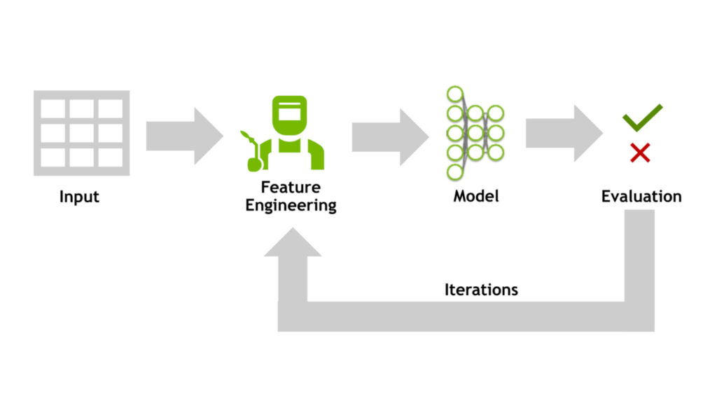
Feature engineering remains one of the most effective ways to improve model accuracy when working with tabular data. Unlike domains such as NLP and computer vision, where neural networks can extract rich patterns from raw inputs, the best-performing tabular models—particularly gradient-boosted decision trees—still gain a significant advantage from well-crafted features. However, the sheer potential number of useful features means that exploring them thoroughly is often computationally prohibitive. Trying to generate and validate hundreds or thousands of feature ideas using standard pandas on a CPU is simply too slow to be practical.
This is where GPU acceleration changes the game. Using NVIDIA cuDF-pandas, which accelerates pandas operations on GPUs with zero code changes, allowed me to rapidly generate and test over 10,000 engineered features for Kaggle’s February playground competition. This accelerated discovery process was the key differentiator. In a drastically reduced timeframe – days instead of potential months –?the best 500 discovered features significantly boosted the accuracy of my XGBoost model, securing 1st place in the competition predicting backpack prices. Below, I share the core feature engineering techniques, accelerated by cuDF-pandas, that led to this result.
Groupby(COL1)[COL2].agg(STAT)
The most powerful feature engineering technique is groupby aggregations. Namely, we execute the code groupby(COL1)[COL2].agg(STAT). This is where we group by COL1 column and aggregate (i.e. compute) a statistic STAT over another column COL2. We use the speed of NVIDIA cuDF-Pandas to explore thousands of COL1, COL2, STAT combinations. We try statistics (STAT) like “mean”, “std”, “count”, “min”, “max”, “nunique”, “skew” etc etc. We choose COL1 and COL2 from our tabular data’s existing columns. When COL2 is the target column, then we use nested cross-validation to avoid leakage in our validation computation. When COL2 is the target, this operation is called Target Encoding.
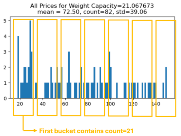
Groupby(COL1)[‘Price’].agg(HISTOGRAM BINS)
When we groupby(COL1)[COL2] we have a distribution (set) of numbers for each group. Instead of computing a single statistic (and making one new column), we can compute any collection of numbers that describe this distribution of numbers and make many new columns together.
Below we display a histogram for the group Weight Capacity = 21.067673. We can count the number of elements in each (equally spaced) bucket and create a new engineered feature for each bucket count to return to the groupby operation! Below we display seven buckets, but we can treat the number of buckets as a hyperparameter.
result = X_train2.groupby("WC")["Price"].apply(make_histogram)X_valid2 = X_valid2.merge(result, on="WC", how="left") |
Groupby(COL1)[‘Price’].agg(QUANTILES)
We can groupby and compute the quantiles for QUANTILES = [5,10,40,45,55,60,90,95] and return the eight values to create eight new columns.
for k in QUANTILES: result = X_train2.groupby('Weight Capacity (kg)').\ agg({'Price': lambda x: x.quantile(k/100)}) |
All NANs as Single Base-2 Column
We can create a new column from all the NANs over multiple columns. This is a powerful column which we can subsequently use for groupby aggregations or combinations with other columns.
train["NaNs"] = np.float32(0)for i,c in enumerate(CATS): train["NaNs"] += train[c].isna()*2**i |
Put Numerical Column into Bins
The most powerful (predictive) column in this competition is Weight Capacity. We can create more powerful columns based on this column by binning this column with rounding.
for k in range(7,10): n = f"round{k}" train[n] = train["Weight Capacity (kg)"].round(k) |
Extract Float32 as Digits
The most powerful (predictive) column in this competition is Weight Capacity. We can create more powerful columns based on this column by extracting digits. This technique seems weird, but it is often used to extract info from a product ID where individual digits within a product ID convey info about a product such as brand, color, etc.
for k in range(1,10): train[f'digit{k}'] = ((train['Weight Capacity (kg)'] * 10**k) % 10).fillna(-1).astype("int8") |
Combination of Categorical Columns
There are eight categorical columns in this dataset (excluding numerical column Weight Capacity). We can create 28 more categorical columns by combining all combinations of categorical columns. First, we label encode the original categorical column into integers with -1 being NAN. Then we combine the integers:
for i,c1 in enumerate(CATS[:-1]): for j,c2 in enumerate(CATS[i+1:]): n = f"{c1}_{c2}" m1 = train[c1].max()+1 m2 = train[c2].max()+1 train[n] = ((train[c1]+1 + (train[c2]+1)\ /(m2+1))*(m2+1)).astype("int8") |
Use Original Dataset which Synthetic Data is Created From
We can treat the original dataset that this competition’s synthetic data was created from as the manufacturer suggested retail. And treat this competition’s data as the individual stores’ prices. Therefore, we can help predictions by giving each row knowledge of the MSRP:
tmp = orig.groupby("Weight Capacity (kg)").Price.mean()tmp.name = "orig_price"train = train.merge(tmp, on="Weight Capacity (kg)", how="left") |
Division Features
After creating new columns with groupby(COL1)[COL2].agg(STAT), we can then combine these new columns to make even more new columns. For example:
# COUNT PER NUNIQUEX_train['TE1_wc_count_per_nunique'] =\ X_train['TE1_wc_count']/X_train['TE1_wc_nunique']# STD PER COUNTX_train['TE1_wc_std_per_count'] =\ X_train['TE1_wc_std']/X_train['TE1_wc_count'] |
Summary
The first place result in this Kaggle competition wasn’t just about finding the right features – it was about having the speed to find them. Feature engineering remains essential for maximizing tabular model performance, but the traditional approach using CPUs often hits a wall, making extensive feature discovery prohibitively slow.
NVIDIA cuDF-pandas is changing what is possible. By accelerating pandas operations on the GPU, it enables the mass exploration and generation of new features in drastically reduced timeframes. This allows us to find the best features and build more accurate models than before. View the solution’s source code and associated Kaggle discussion posts here and here.
If you’d like to learn more, check out our GTC 2025 workshop on Feature Engineering or Bring Accelerated Computing to Data Science in Python, or enroll in our DLI Learning Path courses for data science.