
Workloads processing large amounts of data, especially those running on the cloud, will often use an object storage service (S3, Google Cloud Storage, Azure Blob Storage, etc.) as the data source. Object storage services can store and serve massive amounts of data, but getting the best performance can require tailoring your workload to how remote object stores behave. This post is for RAPIDS users who want to read or write data to object storage as quickly as possible so that IO doesn’t bottleneck your workload.
Some of your knowledge about how local file systems behave translates to remote object stores, but they are fundamentally different. Probably the biggest difference between the two, at least for data analysis workloads, is that read and write operations on object storage have higher and more variable latency. Every storage service has their own set of best practices and performance guidelines (AWS, Azure). Here, we’ll give some general guidelines that are focused on data analysis workloads.
Location
Placing your compute nodes near the storage service (ideally, in the same cloud region) will give you the fastest and most reliable network between the machines running your workload and the machines serving the data. And, at the end of the day, the transfer will be limited by the speed of light so minimizing the physical distance doesn’t hurt.
File format
“Cloud-native” file formats have been developed to work well with object storage. These file formats typically provide fast, easy access to metadata (which includes both high-level information like the column names or data types, and lower-level information like where in the file specific data subsets are located). Apache Parquet, Zarr, and Cloud Optimized GeoTIFF are some examples of cloud-native file formats for various types of data.
Because object storage services typically support range requests, clients (like cuDF) can read the metadata and then download just the data you actually need. For example, cuDF can read just a few columns out of a Parquet file with many columns, or a Zarr client can read a single chunk out of a large n-dimensional array. These reads are done in just a few HTTP requests, and without needing to download a bunch of extraneous data that just gets filtered out.
File size
Because every read operation requires (at least) one HTTP request, we’d prefer to amortize the overhead from each HTTP request over a reasonably large number of bytes. If you control the data-writing process, you’ll want to ensure that the files are large enough for your downstream processing tasks to get good performance. The optimal value depends on your workload, but somewhere in the dozens to low-hundreds of MBs is common for parquet files (see below for some specific examples).
That said, you’ll need to be careful with how file size interacts with the next tool in our kit: concurrency.
Concurrency
Using concurrency to download multiple blobs (or multiple pieces of a single blob) at the same time is essential to getting good performance out of a remote storage service. Since it’s a remote service, your process is going to spend some time (perhaps a lot of time) waiting around doing nothing. This waiting spans the time between when the HTTP request is sent and the response received. During this time, we wait for the network to carry the request, the storage service to process it and send the response, and the network to carry the (possibly large) response. While parts of that request/response cycle scale with the amount of data involved, other parts are just fixed overhead.
Object storage services are designed to handle many concurrent requests. We can combine that with the fact that each request involves some time waiting around doing nothing, to make many concurrent requests to raise our overall throughput. In Python, this would typically be done using a thread pool:
pool = concurrent.futures.ThreadPoolExecutor()futures = pool.map(request_chunk, chunks) |
Or with asyncio:
tasks = [request_chunk_async(chunk) for chunk in chunks]await asyncio.gather(*tasks) |
We’re able to have a lot of reads waiting around doing nothing at the same time, which improves our throughput. Because each thread/task is mostly doing nothing, it’s ok to have more threads/tasks than your machine has cores. Given enough concurrent requests you will eventually saturate your storage service, which has some requests per second and bandwidth targets it tries to meet. But those targets are high; you’ll typically need many machines to saturate the storage service and should achieve very high throughput.
Libraries
Everything above applies to essentially any library doing remote IO from an object storage service. In the RAPIDS context, NVIDIA KvikIO is notable because
- It automatically chunks large requests into multiple smaller ones and makes those requests concurrently.
- It can read efficiently into host or device memory, especially if GPU Direct Storage is enabled.
- It’s fast.
As mentioned in the RADIDS 24.12 release announcement, KvikIO can achieve impressive throughput when reading from S3. Let’s take a look at some benchmarks to see how it does.
Benchmarks
When you read a file, KvikIO splits that read into smaller reads of kvikio.defaults.task_size bytes. It makes those read requests in parallel using a thread pool with kvikio.defaults.num_threads workers. These can be controlled using the environment variables KVIKIO_TASK_SIZE and KVIKIO_NTHREADS, or through Python with:
with kvikio.defaults.set_num_threads(num_threads), kvikio.defaults.set_task_size(size): ... |
See Runtime Settings for more.
This chart shows the throughput, in megabits per second, of reading a 1 GB blob from S3 to a g4dn EC2 instance in the same region for various sizes of the thread pool (higher is better).
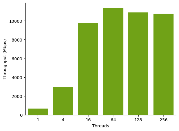
kvikio.RemoteFile.read for various values of kvikio.defaults.num_threads and a task size of 16 MiB. Throughput increases as we add more threads and parallelize the reads, up to a point.Fewer threads (less than four) achieve lower throughput and take longer to read the file. More threads (64, 128, 256) achieve higher throughput by parallelizing the requests to the storage service, which serves them in parallel. There are diminishing and even negative returns as we hit the limits of the storage service, network, or other bottlenecks in our system.
With remote IO, each thread spends a relatively long time idle waiting for the response, so a higher number of threads (relative to your number of cores) might be appropriate for your workload. We see that the throughput is highest between 64 to 128 threads in this case.
As shown in the next figure, the task size also affects the maximum throughput.
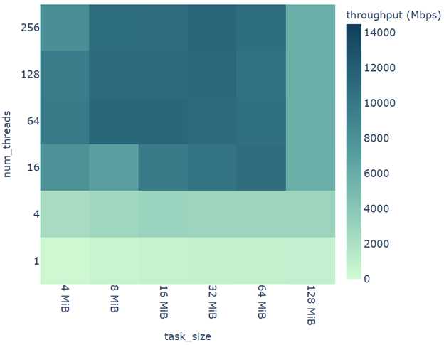
kvikio.RemoteFile.read. The horizontal axis shows throughput for various task sizes, while the vertical axis shows various thread counts.As long as the task size isn’t too small (around or below 4 MiB) or too large (around or above 128 MiB), then we get around 10 Gbps of throughput. With too small of a task size, the overhead of making many HTTP requests reduces throughput. With too large of a task size, we don’t get enough concurrency to maximize throughput.
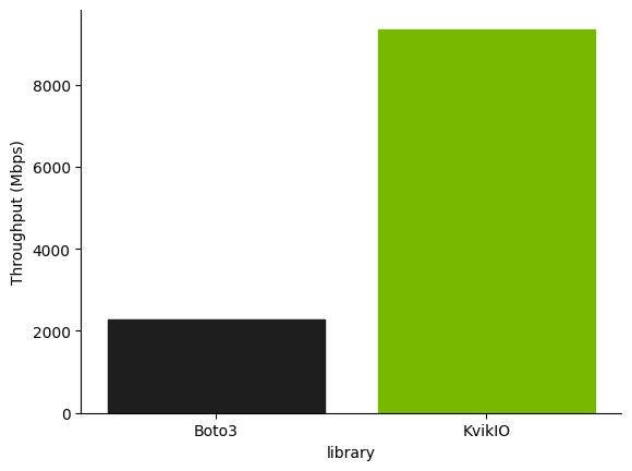
KvikIO achieves higher throughput on this workload when compared with boto3, the AWS SDK for Python, even when boto3 is used in a thread pool to execute requests concurrently.
As a slightly more realistic workload, though still just one focused solely on IO, we compare the performance reading a batch of 360 parquet files, each about 128 MB. This was run on an AWS g4dn.12xlarge instance, which has 4 NVIDIA T4 GPUs and 48 vCPUs.
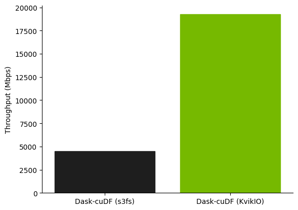
With KvikIO enabled, the four Dask worker processes are able to collectively achieve almost 20 Gbps of throughput from S3 to this single node.
Conclusion
As RAPIDS accelerates other parts of your workload, IO can become a bottleneck. If you’re using object storage and are tired of waiting around for your data to load, try out some of the recommendations from this post. Let us know how things work with KvikIO on GitHub. You can also join over 3,500 members on the RAPIDS Slack community to talk GPU-accelerated data processing.