As PyData leverages much of the static language world for speed including CUDA, we need tools which not only profile and measure across languages but also devices, CPU, and GPU. While there are many great profiling tools within the Python ecosystem: line-profilers like cProfile and profilers which can observe code execution in C-extensions like PySpy/Viztracer. None of the Python profilers can profile code running on the GPU. Developers need tooling to help debug/profile and generally understand what is happening on the GPU from Python. Fortunately, such tooling exists — NVIDIA Tools Extension (NVTX) and Nsight Systems together are powerful tools for visualizing CPU and GPU performance.
NVTX is an annotation library for code in multiple languages, including Python, C, C++. We can use Nsight Systems to trace standard Python functions, PyData libraries like Pandas/NumPy, and even the underlying C/C++ code of those same PyData libraries! Nsight Systems also ships with additional hooks for CUDA to give developers insight to what is happening on the device (on the GPU). This means we can “see” CUDA calls like cudaMalloc, cudaMemcpy, etc.
Quick Start
NVTX is a code annotation tool and can be used to mark functions or chunks of code. Python developers can either use decorators @nvtx.annotate()or a context manager with nvtx.annotate(..): to mark code to be measured. For example:
import time
import nvtx


@nvtx.annotate(“f()”, color="purple")
def f():
    for i in range(5):
        with nvtx.annotate("loop", color="red"):
            time.sleep(i)

f()
Annotating code by itself doesn’t achieve anything. To get information about the annotated code, we typically need to run it with a third-party application such as NVIDIA Nsight Systems. In the above, we’ve annotated a function, f, and a for loop. We can then run the program with Nsight Systems CLI:

> nsys profile -t nvtx,osrt --force-overwrite=true --stats=true --output=quickstart python nvtx-quickstart.py
The option -t nvtx,osrt defines what nsys should capture. In this case, nvtx annotations and OS RunTime (OSRT) functions (read/select/etc).
After both nsys and the python program finish, two files are generated: a qdrep file and a sqlite database. We can visualize the timeline of the workflow by loading the qdrep file with Nsight Systems UI (available on all OSes)
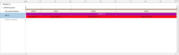
Value of a timeline view
At first glance this isn’t the most exciting profile — the code itself is uncomplicated. But unlike other profiling tools, this view is a timeline. This means we can better evaluate end-to-end workflows and introspect code as the workflow proceeds and not just how much time total we speed in loop or f(). Though nsys also present that view as well
NVTX Push-Pop Range Statistics (nanoseconds)
| Time(%) | Total Time. | Instance | Average | Minimum | maximum Range |
| 50.0 | 10009044198 | 1 | 10009044198.0 | 10009044198 | 10009044198 f |
| 50.0 | 10008769086 | 5 | 2001753817.2 | 4293 | 4002451694 loop |
Like py-spy, NVTX can also profile across multiple processes and threads.
@nvtx.annotate("mean", color="blue")
def compute_mean(x):
    return x.mean()

@nvtx.annotate("mock generate data", color="red")
def read_data(size):
    return np.random.random((size, size))

def big_computation(size):
    time.sleep(0.5)  # mock warmup
    data = read_data(size)
    return compute_mean(data)

@nvtx.annotate("main")
def main():
    ctx = multiprocessing.get_context("spawn")
    sizes = [4096, 1024]
    procs = [
        ctx.Process(name="calculate", target=big_computation, args=[sizes[i]])
        for i in range(2)
    ]

    for proc in procs:
        proc.start()

    for proc in procs:
        proc.join()
We can then run the program with Nsight Systems CLI:
> MKL_NUM_THREADS=1 OPENBLAS_NUM_THREADS=1 OMP_NUM_THREADS=1 nsys profile -t nvtx,osrt,cuda --stats=true --force-overwrite=true --output=multiprocessing python nvtx-multiprocess.py
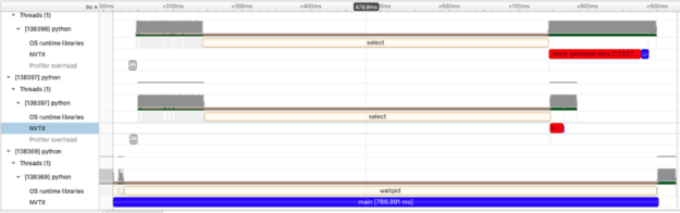
In this example, we create two processes to create a large amount of data and compute the mean. In the first process we build a 4096×4096 matrix of random data and in the second process, a 1024×1024 matrix of random data. What we see in the visualization are two red bars (noting the data creation time and 3 blue bars (though admittedly the blue bar attached to the small red data generation task is hard to see). We see two very informative things here which can be hard to capture in tools which only measure time spent:
- The processes overlap in time and we see the data generation of both matrices occurring at the same time!
- Data generation cost is non-zero and the large 4096×4096 matrix takes considerably more time as does the calculation of mean.
Annotation across GPUs (Cuda specific)
An Nsight Systems’ feature called “NVTX range protection allows user to annotate across devices, specifically NVIDIA GPUs. This means we can develop a deep understanding of not just what is happening on the GPU itself (cudaMalloc, Compute Time, Synchronization), but also leverage the GPU from Python in a diverse, complicated, multi-threaded, multi-process, multi-library landscape. Again, let’s ease our way in.
with nvtx.annotate("data generation", color="purple"):
     imgs = [cupy.random.random((1024, 1024)) for i in range(100)]
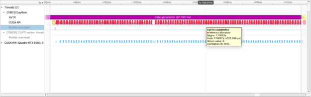
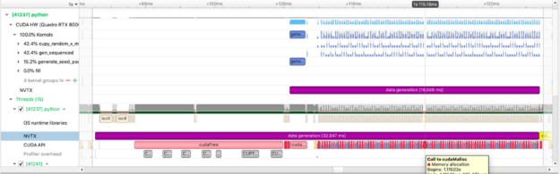
We use CuPy, a NumPy-like library targeting GPUs, to operate on the data just as we do with NumPy data. The figure above captures how long we spend allocating data on the GPU.We can also see the execution of individual cupy kernels: cupy_random, gen_sequence, generate_seed as well as where and when the kernels are executed relative to other operations.The example below calculates the squared difference between two matrices and measures the time spent performing this calculation:
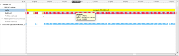
def squared_diff(x, y):
    return (x - y) * (x - y)

with nvtx.annotate("compute", color="yellow"):
    squares = [squared_diff(arr_x, arr_y) for arr_x, arr_y in list(zip(imgs, imgs[1:]))]
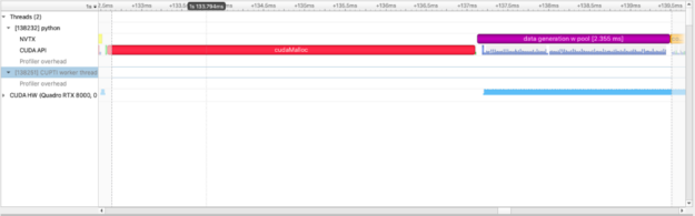
Using a pool allocator for performance
With this information, we can now visually understand how and where the GPU spends time. Next, we can ask, can we do better? The answer is YES! cudaMalloc is a non-zero time operation and creating many GPU allocations can negatively impact performance. Instead, we can use the RAPIDS RMM pool allocator which will create a large upfront GPU memory allocation and allow us to make sub-allocations at significantly faster speeds:
cupy.cuda.set_allocator(rmm.rmm_cupy_allocator)
rmm.reinitialize(pool_allocator=True, initial_pool_size=2 ** 32)  # 4GBs

with nvtx.annotate("data generation w pool", color="purple"):
    imgs = [cupy.random.random((1024, 1024)) for i in range(100)]
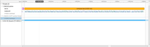
For this particular operation, squared_difference, we can use cupy.fuse to optimize elementwise kernels. This is a common GPU optimization.
with nvtx.annotate("compute fast", color="orange"):
    squares = [
        cupy.fuse(squared_diff(arr_x, arr_y))
        for arr_x, arr_y in list(zip(imgs, imgs[1:]))
    ]
NVTX helps developers and users
The annotations themselves have minimal overhead and only capture information when executed with nsys. Profiling code provides useful information to users and developers that is otherwise hidden and reveals much about where and why time is being spent. When library authors choose to annotate with NVTX, users can develop a more complete understanding of end-to-end workflows For example, with RAPIDS cuDF, a GPU Dataframe library, kernels will often need to allocate memory as part of group by-aggregation. As we saw before using the RMM pool allocator will reduce the amount of time spent creating GPU memory:
rmm.reinitialize(pool_allocator=True, initial_pool_size=2 ** 32)  # 4GBs

gcdf1 = cdf1.groupby("id").mean().reset_index()
gcdf2 = cdf2.groupby("id").mean().reset_index()

gcdf2.join(gcdf1, on=["id"], lsuffix="_l")
We can also quickly see why some equivalent operations are faster than others depending on the route taken. When performing several groupby-aggregations (groupby().mean(), groupby().count(), …), we can either perform each individually or use the agg operator. Using agg will only perform the groupby operation once.
with nvtx.annotate("agg-all", color="blue"):
    cdf.groupby("name").agg(["count", "mean", "sum"])

with nvtx.annotate("split-agg", color="red"):
    cdf.groupby("name").count(), cdf.groupby("name").mean(), cdf.groupby("name").count()
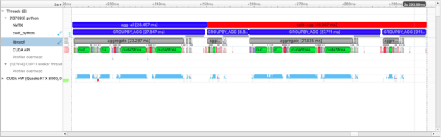
In the plot above we see more than the agg-all and split-agg annotations. We see the annotations inserted by cuDF developers and can clearly see one group-agg call for agg(["count", "mean", "sum"]) and three group-agg calls for count(), mean(), sum().
Next Steps
Currently, annotating a function within a package requires users to make modifications to that package, or convince the maintainer(s) to annotate parts of the package. It would be convenient to be able to annotate a function without modifying its source code. It’s not immediately clear how to achieve this.
Another potentially useful feature would be to annotate execution threads. Currently, the different threads of execution are named Thread 0, Thread 1, etc., which may not be as useful. This is already possible in the C layer, but not exposed in the Python layer currently.
While these are just a few thoughts on our minds, we would welcome suggestions from the community. We maintain a GitHub repo with the C, C++, and Python bindings and would welcome issues on the issue tracker. If there are things missing, we welcome PRs and are happy to review. Also, just drop by and say hi, we have a Slack channel as well.
Conclusion
It’s easy to download NVTX using pip or conda:
python -m pip install nvtx
or:
conda install -c conda-forge nvtx
The examples from this blog post (and a few others) are available at this GitHub repository.