上一篇文章“How to Accelerate Quantitative Finance with ISO C++ Standard Parallelism”(如何使用 ISO C++標準并行機制加速量化金融) 演示了如何使用 ISO C++標準并行機制和NVIDIA accelerated-quant-finance GitHub 庫中找到的代碼編寫 Black-Scholes 模擬。這種方法使您能夠高效地編寫簡潔且可移植的代碼。
僅使用標準 C++,就可以編寫可在現代多核 CPU 或 GPU 上并行運行的應用程序,而無需進行修改。本文從之前開發的 Black-Scholes 并行代碼開始,構建了一個更復雜的模型,并對其進行了優化,以利用 GPU 的優勢,同時保留標準 C++。
利潤和損失建模說明
交易已實現波動性的熱門策略是對期權持倉進行增量套期保值。根據 Black-Scholes 的假設,如果投資者成功套期保值了基礎風險,則此策略的主要盈利和損失因素(P&L)與已實現波動性的平方與用于定價和套期保值的波動性之間的差值成比例。
市盈率取決于底層資產的路徑。估算大型期權組合在給定水平線上的完整市盈率分布可能需要大量計算,因此需要擴展并行 Black-Scholes 代碼。
考慮在同一底層資產上由各種執行力和到期日組成的多頭歐洲看漲期權網格?


隨著時間的推移,底層
對于給定的期權合約,權利金是多個參數的函數,其中包括 
假設所有參數隨著時間推移保持不變,則選項會隨著時鐘的每個刻度而失去值。隨著時間推移,選項值的這種負變化稱為 theta 或時間衰減。
作為底層
首先,期權值的變化由增量選項的值。例如,如果增量為 0.55 并且
其次,
在增量套期保值選項的情況下,總增量 delta P&L 為零,而 gamma 增益有可能抵消、超過或承受由于 theta 而造成的損失 (圖 1)。

在本示例中,目標是通過模擬底層資產的路徑并沿這些路徑累加 P&L,描述網格中每個選項在給定水平下的 gamma-theta P&L 分布。
在這個簡單的 Black-Scholes 世界中,底層資產在風險中性測量下遵循對數正態動力學,并實現了波動性?

每日 (或一次性步驟) 盈利和損失可通過以下方式獲得:

在這個方程中,?


底層資產的單個路徑上的損失,包括

并行 P&L 模擬
圖 2 顯示了選項網格和四個模擬路徑。每個網格單元代表一個期權合約,其相應的貨幣性和成熟時間分別標記在水平軸和垂直軸上。熱圖中的顏色與這些路徑中的平均 P&L 成正比。平均值只是一個統計量,可以從模擬的 P&L 中計算,該 P&L 可通過模擬獲得完整分布。

上一篇文章中的并行代碼用作基準。每個路徑都循環遍歷,然后行走,正如之前的示例中所做的那樣,將選項的P&L計算并行化。
這是一種合理的方法,因為有可能有大量選項進行并行化。代碼本身很簡單,唯一的主要區別是在最后添加了一個transform,以將總和轉換為均值。
但是,仍有機會進一步優化代碼并提高性能。
void calculate_pnl_paths_sequential(stdex::mdspan<const double, stdex::dextents<size_t,2>> paths, std::span<const double>Strikes, std::span<const double>Maturities, std::span<const double>Volatilities, const double RiskFreeRate, std::span<double>pnl, const double dt){ int num_paths = paths.extent(0); int horizon = paths.extent(1); auto steps = std::views::iota(1,horizon); // Iterate from 0 to num_paths - 1 auto path_itr = std::views::iota(0,num_paths); // Note - In this version path remains in CPU memory // Note - Also that when built for the GPU this will result in // num_paths * (horizon - 1) kernel launches std::for_each(path_itr.begin(), path_itr.end(), [=](int path) // Called for each path from 0 to num_paths - 1 { // Iterate from 1 to horizon - 1 std::for_each(steps.begin(), steps.end(), [=](int step) // Called for each step along the chosen path { // Query the number of options from the pnl array int optN = pnl.size(); // Enumerate from 0 to (optN - 1) auto opts = std::views::iota(0,optN); double s = paths(path,step); double s_prev = paths(path,step-1); double ds2 = s - s_prev; ds2 *= ds2; // Calculate pnl for each option std::transform(std::execution::par_unseq, opts.begin(), opts.end(), pnl.begin(), [=](int opt) { double gamma = 0.0, theta = 0.0; BlackScholesBody(gamma, s_prev, Strikes[opt], Maturities[opt] - std::max(dt*(step-1),0.0), RiskFreeRate, Volatilities[opt], CALL, GAMMA); BlackScholesBody(theta, s_prev, Strikes[opt], Maturities[opt] - std::max(dt*(step-1),0.0), RiskFreeRate, Volatilities[opt], CALL, THETA); // P&L = 0.5 * Gamma * (dS)^2 + Theta * dt return pnl[opt] + 0.5 * gamma * ds2 + (theta*dt); }); }); });} |
提高并行性以提高性能
每當將并行算法卸載到 GPU 時,都會產生兩種用度:
- 啟動延遲:啟動 GPU 內核的成本。
- 同步:并行算法相對于 CPU 是同步的,這意味著程序必須等待內核完成,然后再繼續并啟動下一個內核。
這兩種開銷都不是特別大,每次都只有一小部分秒,但當重復執行時,開銷會增加。更糟糕的是,NVIDIA Nsight Systems 分析器顯示,每個內核都需要比內核本身更長的設備同步步驟。
路徑是獨立的隨機行走,除了底層計算的相同初始值之外,沒有任何關系?
要解決這種潛在的競爭狀況,請使用 C++atomic_ref以確保如果兩條路徑嘗試同時更新 P&L 數組中的同一位置,它們將以安全的方式執行此操作。
通過將路徑的迭代轉移到函數中,現在可以在每個路徑的路徑和選項上實現并行化。雖然這個示例更復雜,但它本質上與為初始示例所做的重構相同。
void calculate_pnl_paths_parallel(stdex::mdspan<const double, stdex::dextents<size_t,2>> paths, std::span<const double>Strikes, std::span<const double>Maturities, std::span<const double>Volatilities, const double RiskFreeRate, std::span<double>pnl, const double dt){ int num_paths = paths.extent(0); int horizon = paths.extent(1); int optN = pnl.size(); // Create an iota to enumerate the flatted index space of // options and paths auto opts = std::views::iota(0,optN*num_paths); std::for_each(std::execution::par_unseq, opts.begin(), opts.end(), [=](int idx) { // Extract path and option number from flat index // C++23 cartesian_product would remove the need for below int path = idx/optN; int opt = idx%optN; // atomic_ref prevents race condition on elements of pnl array. std::atomic_ref<double> elem(pnl[opt]); // Walk the path from 1 to (horizon - 1) in steps of 1 auto path_itr = std::views::iota(1,horizon); // Transform_Reduce will apply the lambda to every option and perform // a plus reduction to sum the PNL value for each option. double pnl_temp = std::transform_reduce(path_itr.begin(), path_itr.end(), 0.0, std::plus{}, [=](int step) { double gamma = 0.0, theta = 0.0; double s = paths(path,step); double s_prev = paths(path,step-1); double ds2 = s - s_prev; ds2 *= ds2; // Options in the grid age as the simulation progresses // along the path double time_to_maturity = Maturities[opt] – std::max(dt*(step-1),0.0); BlackScholesBody(gamma, s_prev, Strikes[opt], time_to_maturity, RiskFreeRate, Volatilities[opt], CALL, GAMMA); BlackScholesBody(theta, s_prev, Strikes[opt], time_to_maturity, RiskFreeRate, Volatilities[opt], CALL, THETA); // P&L = 0.5 * Gamma * (dS)^2 + Theta * dt return 0.5 * gamma * ds2 + (theta*dt); }); // accumulate on atomic_ref to pnl array elem.fetch_add(pnl_temp, std::memory_order_relaxed); });} |
std::for_each算法用于在路徑和選項之間進行迭代。在每次迭代中,std::transform_reduce算法用于遍歷每個選項的每個路徑,將利潤和損失相加并返回該結果。然后,每個中間結果都會自動添加到 P&L 數組中。
此方法的主要優點是,無需在 GPU 和 CPU 之間反復來回反彈,而是在 GPU 上針對完整數據集啟動單個操作,且程序僅需等待一次結果(圖 3)。

這種方法的性能比原始版本顯著提升,而原始版本本身已在 GPU 上加速(圖 4)。

從第二個示例中汲取的經驗是,盡可能多地展示硬件的并行性。第一種方法改進了 CPU 和 GPU 版本,但 GPU 版本在通過更多并行性減少啟動和同步開銷后確實非常出色。
探索代碼
使用 NVIDIA accelerated-quant-finance GitHub 庫中的代碼在此量化金融示例中實現的加速可輕松應用于 C++ 應用程序。使用串行循環編寫的任何 C++ 代碼都可以使用標準語言并行輕松修改,以實現顯著的 GPU 加速。
要輕松生成自己的可移植并行優先代碼,請下載 NVIDIA HPC SDK,其中包含利用 ISO C++ 標準并行性并對結果進行分析的所有工具。
?